Example: Wide and Long Format
The following is a short note on converting wide to long format required e.g. for some lattice or ggplot visualizations. The following examples are based on the readily known data set showing the percentage fraction of settlement, recreational, agricultural, and forest areas for each rural district in Germany. The data has been provided through the Regional Database Germany.
## Loading required package: reshape2
## Loading required package: car
## Loading required package: carData
## Loading required package: plotly
## Loading required package: ggplot2
##
## Attaching package: 'plotly'
## The following object is masked from 'package:ggplot2':
##
##     last_plot
## The following object is masked from 'package:stats':
##
##     filter
## The following object is masked from 'package:graphics':
##
##     layout
## Loading required package: forecast
## Loading required package: zoo
##
## Attaching package: 'zoo'
## The following objects are masked from 'package:base':
##
##     as.Date, as.Date.numeric
## Loading required package: TSA
##
## Attaching package: 'TSA'
## The following objects are masked from 'package:stats':
##
##     acf, arima
## The following object is masked from 'package:utils':
##
##     tar
## Loading required package: Kendall
## Loading required package: dtw
## Loading required package: proxy
##
## Attaching package: 'proxy'
## The following objects are masked from 'package:stats':
##
##     as.dist, dist
## The following object is masked from 'package:base':
##
##     as.matrix
## Loaded dtw v1.20-1. See ?dtw for help, citation("dtw") for use in publication.
## Loading required package: TSclust
## Loading required package: wmtsa
## Loading required package: pdc
## Loading required package: cluster
## Loading required package: lattice
## Loading required package: RColorBrewer
##
## Attaching package: 'latticeExtra'
## The following object is masked from 'package:ggplot2':
##
##     layer
library(latticeExtra)
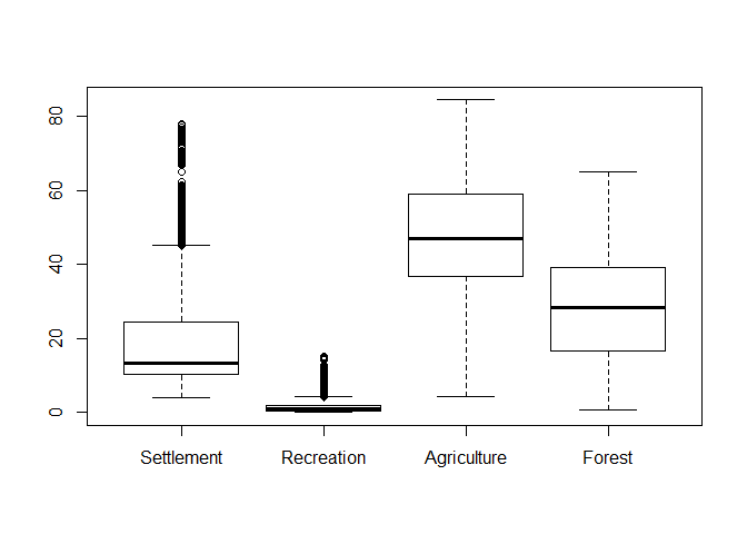
We already know that a boxplot is probably the most fundamental way to perform a visual data exploration. Producing it is straight forward in generic plotting: Producing a boxplot is staright forward (the x-axis lables are just the column names):
boxplot(lu[, c("Settlement", "Recreation", "Agriculture", "Forest")])
Producing a boxplot in lattice is not so staright forward as in generic plotting if you whish to have multiple variables shown in one plot. Before one can plot it, one has to transform the data into “long” format. In the case of our dataset, this implies to identify the ID variables (i.e. the ones who define the place and time of the measurement). After this is done, the long-format will duplicate them as often as it is required to fit in all values of the other columns (i.e. setellment, recreation, agriculture and forest) and add the respective values in a seperate column.
That’s what the data looks like in it’s original format:
head(lu)
##   ID Year                  A          B    C Agriculture Forest Recreation
## 1 01 1996 Schleswig-Holstein Bundesland <NA>        73.0    9.3        0.7
## 2 01 2000 Schleswig-Holstein Bundesland <NA>        72.2    9.5        0.7
## 3 01 2004 Schleswig-Holstein Bundesland <NA>        71.0   10.0        0.8
## 4 01 2008 Schleswig-Holstein Bundesland <NA>        70.0   10.4        0.9
## 5 01 2009 Schleswig-Holstein Bundesland <NA>        69.9   10.5        0.9
## 6 01 2010 Schleswig-Holstein Bundesland <NA>        69.8   10.5        0.9
##   Settlement
## 1       10.8
## 2       11.2
## 3       11.9
## 4       12.4
## 5       12.5
## 6       12.6
And this is the data after conversion to long format using the reshape2::melt function:
lul <- reshape2::melt(lu, id.vars = c("Year", "ID", "A", "B", "C"))
head(lul)
##   Year ID                  A          B    C    variable value
## 1 1996 01 Schleswig-Holstein Bundesland <NA> Agriculture  73.0
## 2 2000 01 Schleswig-Holstein Bundesland <NA> Agriculture  72.2
## 3 2004 01 Schleswig-Holstein Bundesland <NA> Agriculture  71.0
## 4 2008 01 Schleswig-Holstein Bundesland <NA> Agriculture  70.0
## 5 2009 01 Schleswig-Holstein Bundesland <NA> Agriculture  69.9
## 6 2010 01 Schleswig-Holstein Bundesland <NA> Agriculture  69.8
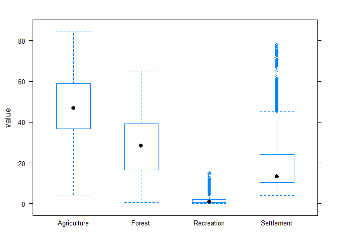
Afterwards, the data can also be used e.g. for producing boxplots in lattice:
bwplot(value ~ variable, data = lul)
Just in case, back to wide format.
lul_wide_again = dcast(lul, ID + Year + A + B + C ~ variable, value.var = "value")
head(lul)
##   Year ID                  A          B    C    variable value
## 1 1996 01 Schleswig-Holstein Bundesland <NA> Agriculture  73.0
## 2 2000 01 Schleswig-Holstein Bundesland <NA> Agriculture  72.2
## 3 2004 01 Schleswig-Holstein Bundesland <NA> Agriculture  71.0
## 4 2008 01 Schleswig-Holstein Bundesland <NA> Agriculture  70.0
## 5 2009 01 Schleswig-Holstein Bundesland <NA> Agriculture  69.9
## 6 2010 01 Schleswig-Holstein Bundesland <NA> Agriculture  69.8