Example: Colours and maps
This is a short example on how to use the hcl colour palette for colouring features of a shapefile.
Load the required packages
library("rgdal")
library("raster")
library("sp")
library("classInt")
Always clean the workspace first
rm(list=ls())
Get helper functions (those from the previous side)
clrs_hcl2 <- function(n) {
  hcl(h = seq(0, 260, length.out = n),
      c = 60, l = seq(10, 90, length.out = n),
      fixup = TRUE)
}

pal <- function(col, border = "transparent", ...) {
  n <- length(col)
  plot(0, 0, type="n", xlim = c(0, 1), ylim = c(0, 1),
       axes = FALSE, xlab = "", ylab = "", ...)
  rect(0:(n-1)/n, 0, 1:n/n, 1, col = col, border = border)
}

# If you want to reverse the colour palette, do it like this
pal(rev(clrs_hcl2(10)))
As example data serve political boundaries of the world
Download the data here or directly from within R.
download.file("https://www.naturalearthdata.com/http//www.naturalearthdata.com/download/50m/cultural/ne_50m_admin_0_countries.zip",
              destfile = "countries.zip")
NaturalEarthData has a nice collection of other free GIS data, too.
Example script for plotting with random colours
## Read in shapefile
world <- rgdal::readOGR("countries/ne_50m_admin_0_countries.shp")
## Do the reality check and plot the map
plot(world)
## make a copy to work with
simple_world <- world
## Show the structure of the attribute table
str(simple_world@data) # 241 features (=polygons) with 94 variables (=fields) each.
Note that the @data slot of a spatial* vector object is a data.frame, so work with it like with a data.frame
## Clear the attribute table
simple_world@data[] <- NULL
str(simple_world@data) # now the attribute table is empty. Only the attribute table, the features remain.
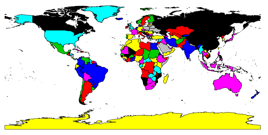
## Let's generate some random values for each feature for plotting later
simple_world@data$random <- sample(1:100, nrow(simple_world@data), replace=TRUE) # note that no seed is set here, so every call will result in a different result
## Use new field with random values for colour plotting
plot(simple_world, col=simple_world@data$random) # fancy and meaningless, but works.
Example script for plotting with classified hcl colours
If we want to do classified plotting, i.e. assign a particular colour to each class, we need to classify our data first and then assign colours to each class.
## Choose the number of desired classes
n <- 10

## Classify the randomly generated data (or any numeric attribute) with some method. In this case equaly spaces classed, i.e. all classed have equal widths. See ?classIntervals for more options.
intervalls <- classInt::classIntervals(simple_world@data$random, n = n, style="equal")

intervalls$brks # shows the calculated breaks

## Assign each class within the feature the a colour according to the previous classification. The colours are produced with the self-defined clrs_hcl2() function from above. Execute all parts of the code line below to see what they do and what they contain.
colours <- classInt::findColours(intervalls, rev(clrs_hcl2(n)), cutlabels=FALSE) # Noteworthy, the values of the object "colours" are the colours definded in the hexadecimal system and there are as many entries as there are values in the original data (attribute "random" in this case). One colour for each value.

## Add the colour code to the attribute table of the spatial object
simple_world@data$colours <- colours

## Use the new field with the colour code for plotting
plot(simple_world, col = simple_world@data$colours)
legend("topleft", legend = names(attr(colours, "table")),
       fill = attr(colours, "palette"),
       border = attr(colours, "palette"),
       bty = "n", title="Legend", cex=0.45, y.intersp = 0.7)
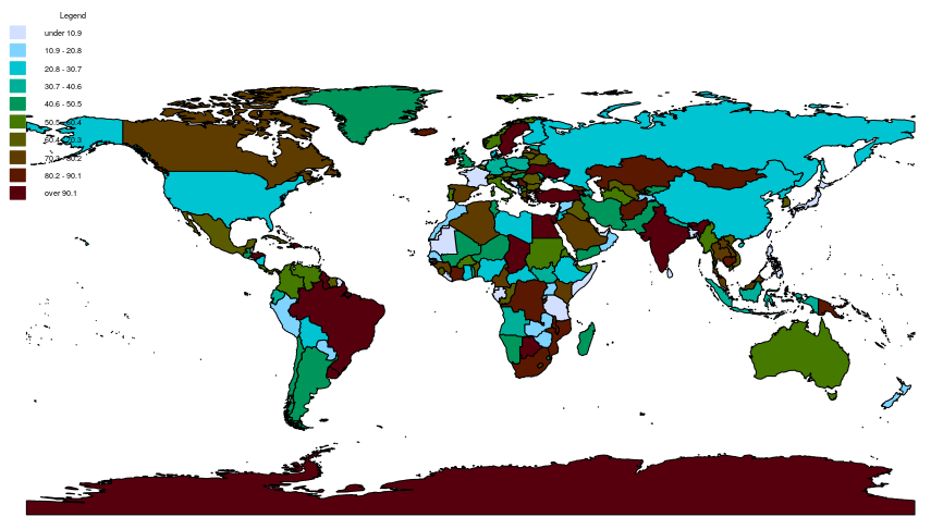
Clearly, the above examples are not ready for publication but intended to demonstrate a schematic workflow for classifying and colouring maps, be it vector or raster.