Spotlight: Artificial Images
Artificial images result from mathematical operations on image data. The operations are pixel or neighborhood based.
Artifical image computations
Artificial images can be used to highlight certain aspects of the spectral information recorded in the original dataset or its horizontal pattern. To compute artificial images, new values have to be calculated for each pixel in the original datasets (original data can be the initially recorded data or any other artificial image which has already been computed). For an extreme example on the utilization of artificial images see e.g. Meyer et al. 2017 who uses over 300 artificial images to estimate their usability in satellite rainfall retrievals.
A list of (minimum) available indices can be found in the Index Data Base of Verena Henrich and Katharina Brüser at Bonn University.
Pixel-wise computation
If the computation is pixel-wise, only those original pixel values are included in the computation at a time which are located at the same position as the respective target pixel. Examples for this type of computation are any kind of spectral index values like the Normalized Different Vegetation Index (NDVI, see this NASA page). A principal component analysis, also based on the entire dataset, can also be regarded as pixel-wise since the final value of e.g. the first principal component at a specific pixel location results from the transformation of the original pixel values at this position.
A special type of pixel-wise computation is the aggregation of LiDAR or other point cloud values into a regular raster and compute information like the minimum or maximum value in this point cloud subset or the number of points etc.
Neighborhood-based computation
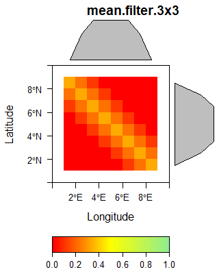
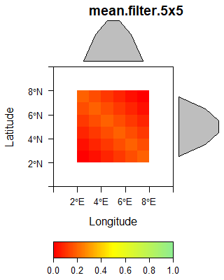
If the computation includes neighboring pixels, the value of the respective target pixel results from a odd number of original pixels located in e.g. a 3 by 3 or 5 by 5 neighborhood of the target pixel including the value of the original pixel in the the center. Examples for this type are any kind of spatial filters, e.g. a standard deviation filter. A prominent group is associated with grey level co-occurence matrix. In general, some filters can not only be based on a single original data layer but a stack of layers.
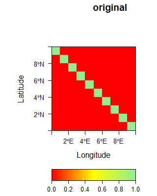
The following gallery shows three examples of spatial filters.
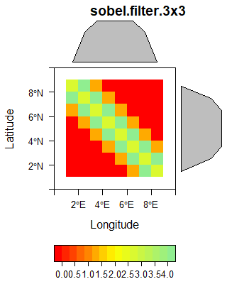
The sobel filter is computed using the following matrix supplied to the raster::focal function.
kx = matrix(c(-1,-2,-1,0,0,0,1,2,1), ncol=3)
ky = matrix(c(1,0,-1,2,0,-2,1,0,-1), ncol=3)
k = (kx**2 + ky**2)**0.5

sobel_raster <- focal(original_raster, w=k)
Morphological feature computation
A second spatial method aims in computing morphological features based on individual raster values. A typical data source is a digital elevation model and typical target datasets are rasters showing the slope, exposition etc. of the surface.
Starting with artifical image computation in R
A good starting point for spatial filtering with R is the raster::focal function for “classic” spatial filtering or the glcm package for grey level co-occurence matrix computations). For the latter, the Orfeo ToolBox offers a large set of Haralick texture computation functions. To link it with R, see the link2GI package and the otbtex_* functions of the uavRst package.