Time series clustering
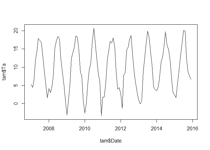
Just as one last example on time series analysis for this module and mainly to demonstrate that this module only tiped a very small set of analysis concepts out there, we will have a glimpse on time series clustering. To illustrate this, we will again use the (mean monthly) air temperature record of the weather station in Coelbe (which is closest to the Marburg university forest). The data has been supplied by the German weatherservice German weather service. For simplicity, we will remove the first 6 entries (July to Dezember 2006 to have full years).
tam <- tam[-(1:6),]
tam$Date <- strptime(paste0(tam$Date, "010000"), format = "%Y%m%d%H%M", tz = "UTC")
plot(tam$Date, tam$Ta, type = "l")
The major risk in time series clustering (or any other clustering) is that one clusters something which actually does not show any kind of groups. Hence, the most important part to remember is that a cluster algorithm will always identify clusters no matter if they are really “exist”. As a consequence: never use clustering if you are not sure that there is a grouping in the data. In addition, clustering is generally applied if you have more than one time series from more than one location.
Of course, there is no rule without exeption and the one exeption is: if you want to show some code and do not want to introduce a new dataset just for this last example, you can use it on a dataset where you have no glimps of a grouping as long as you are not the one who gets the grading in the end.
OK. Aside from having no idea if we have a grouping and aside that we have only a single station record, let’s have a look at the above time series. There might be a difference between 2010 and the rest of the years since 2010 shows very warm summer and cold winter temperatures. To start with clustering, we have to look at the individual years as different time series by transforming our data into a matrix with 12 columns (i.e. one for each month) and the required number of years. Thereby we have to make sure that the original dataset is actually tranformed into the matrix format by rows and not by columns. This will result in a matrix with one year per row:
tam_ta <- matrix(tam$Ta, ncol = 12, byrow = TRUE)
row.names(tam_ta) <- paste0(seq(2007, 2015))
tam_ta
##           [,1]        [,2]      [,3]      [,4]     [,5]     [,6]     [,7]
## 2007  5.268683  4.53095238 6.2369624 11.882361 14.57567 17.89889 17.34704
## 2008  4.178226  3.05474138 4.8426075  7.477222 15.24677 17.32917 18.45255
## 2009 -3.158871  1.30922619 4.8364247 12.364861 14.19651 15.32306 18.52773
## 2010 -2.627823  0.20758929 5.0146505  9.270000 11.06237 17.16667 20.75013
## 2011  1.752285  1.81413690 5.7346774 12.165139 14.15618 17.10208 16.65296
## 2012  2.683468 -1.23189655 7.7043011  8.555278 14.74812 15.57597 17.59153
## 2013  1.092070 -0.04494048 0.7533602  8.902222 12.11250 16.44056 19.96048
## 2014  3.575000  4.64568452 7.0896505 11.548194 12.78562 16.32681 19.79220
## 2015  2.461022  1.62306548 5.0916667  8.785694 12.88306 16.49889 20.10591
##          [,8]     [,9]     [,10]    [,11]      [,12]
## 2007 16.73898 12.67542  8.470296 4.480000  1.6173387
## 2008 17.82917 12.47181  8.755780 5.336667  0.7397849
## 2009 18.33374 14.57264  8.515054 7.857917  0.7282258
## 2010 16.98454 12.57486  8.378898 6.022083 -3.3438172
## 2011 18.06210 15.17806  8.975538 3.989167  4.4114247
## 2012 18.68952 13.27528  8.509005 5.440694  2.8017473
## 2013 18.01801 13.68875 10.692608 4.619167  3.9010753
## 2014 16.05228 14.87569 11.748790 6.533889  3.1159946
## 2015 19.93105 12.79472  8.746774 7.553333  6.7141129
This matrix can subsequently be used to compute the dissimilarity between the individual time series. In this example, we use the TSclust::diss function with method “DTWARP” (which is one of many, each leading to a different result; p gives the decaying of the auto-correlation coefficient to be considered).
tam_dist <- TSclust::diss( tam_ta, "DTWARP", p=0.05)
tam_dist
##          2007     2008     2009     2010     2011     2012     2013
## 2008 19.24069
## 2009 30.79566 31.27686
## 2010 41.22420 39.78805 38.00132
## 2011 22.79959 30.53591 27.06892 42.14468
## 2012 29.35046 21.24988 36.84308 41.79336 31.11600
## 2013 40.45138 40.87593 41.37245 35.56177 25.98853 29.09403
## 2014 26.78914 33.90738 36.86756 40.04724 28.75914 36.35242 32.43355
## 2015 35.82190 30.72825 33.32398 32.51645 28.84693 29.41835 28.72208
##          2014
## 2008
## 2009
## 2010
## 2011
## 2012
## 2013
## 2014
## 2015 29.13347
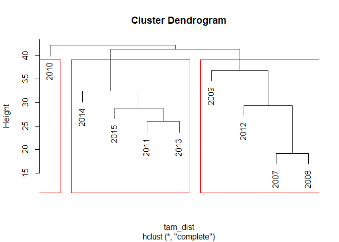
The resulting dissimilarity is larger if the different time series (i.e. years in this case) are less similar and smaller if they are more similar. This dissimillarity is now used for hirachical clustering which computes the distance between the individual samples. Plotting the result shows a cluster dendogram:
tam_hc <- hclust(tam_dist)
plot(tam_hc)
rect.hclust(tam_hc, k = 3)

Just for completness, if you want to derive a certain number of clusters from it, you can use the following for the visualization of the clustres or getting the respective group IDs. In this example, we derive three clusters:
plot(tam_hc)
rect.hclust(tam_hc, k = 3)
cutree(tam_hc, k = 3)
## 2007 2008 2009 2010 2011 2012 2013 2014 2015
##    1    1    1    2    3    1    3    3    3