Generalized additive models
So far, the models have only considered linear relationships. The corresponding model type to simple linear models would be an additive model and for poisson or logistic linear regression, it would be the generalized additive model (GAM). Since (all?) implementations of GAM also allow for additive models (i.e. using gaussian instead of e.g. poisson distribution functions), we will not distinguish between AM and GAM in the following.
To illustrate non-linear fittings, we stay with the anscombe dataset but modify variable x3 and use y1 and y2.
Just for completeness, the following code shows the modification of the anscombe data set although it is not relevant to know anything about it for the examples below:
library(mgcv)
## Loading required package: nlme
## This is mgcv 1.8-24. For overview type 'help("mgcv-package")'.
y <- anscombe$y2
x1 <- anscombe$x1
set.seed(2)
x3 <- anscombe$x3 + sample(seq(-1, 1, 0.1), nrow(anscombe))
y <- c(anscombe$y1, anscombe$y2)
x <- c(x1, x3)
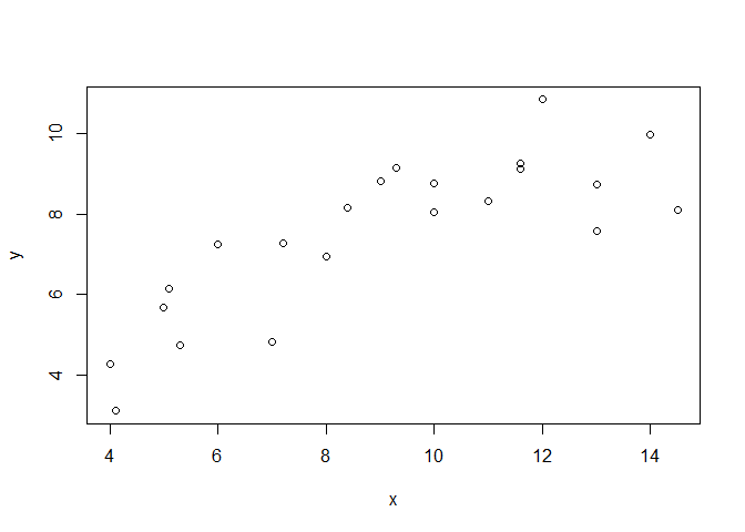
plot(x, y)
df <- data.frame(y = y,
                 x = x)
From linear regression models to generalized additive models
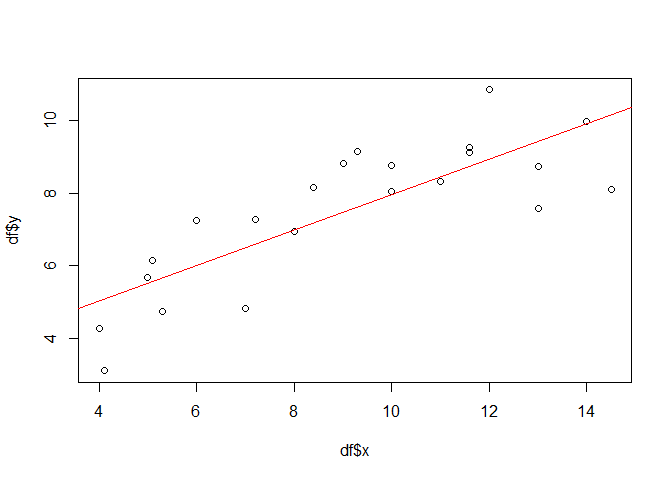
To start with, the following plots shows the data set used within this example and the result of a simple linear regression model.
plot(df$x, df$y)

lmod <- lm(y ~ x, data = df)
abline(lmod, col = "red")
summary(lmod)
##
## Call:
## lm(formula = y ~ x, data = df)
##
## Residuals:
##     Min      1Q  Median      3Q     Max
## -2.0624 -0.7535  0.1160  0.7695  1.8985
##
## Coefficients:
##             Estimate Std. Error t value Pr(>|t|)
## (Intercept)  3.08139    0.75825   4.064 0.000606 ***
## x            0.48834    0.07895   6.185 4.83e-06 ***
## ---
## Signif. codes:  0 '***' 0.001 '**' 0.01 '*' 0.05 '.' 0.1 ' ' 1
##
## Residual standard error: 1.19 on 20 degrees of freedom
## Multiple R-squared:  0.6567,	Adjusted R-squared:  0.6395
## F-statistic: 38.26 on 1 and 20 DF,  p-value: 4.833e-06
Provided that all the assumptions relevant for linear models are met, x is significant and the model explains about 0.6567 percent of the variation in the data set.
One might think that replacing lm with mgcv:gam (i.e. the gam function from the mgcv package) would be enough to turn our model in an additive model. However, this is not true. In fact, gam with (it’s default) gaussian family acts exactly as the lm function if the same forumla is supplied. We will show this by plotting the gam-based regression line (dotted, red) on top of the one from the linear model above (grey).
gammod <- gam(y ~ x, data = df, familiy = gaussian())

px <- seq(min(df$x), max(df$x), 0.1)
gampred <- predict(gammod, list(x = px))

plot(df$x, df$y)
abline(lmod, col = "grey")
lines(px, gampred, col = "red", lty=2)

No difference. Although we need some more code since we have to predict the model values before we can overlay them in the plot. Therefore, the vector px is used and initialized with a sequence between the minimum and maximum x value and a step of 0.1. This is also sufficient to visualize more “non-linear” model predictions later.
Let’s have a look at the summary:
summary(gammod)
##
## Family: gaussian
## Link function: identity
##
## Formula:
## y ~ x
##
## Parametric coefficients:
##             Estimate Std. Error t value Pr(>|t|)
## (Intercept)  3.08139    0.75825   4.064 0.000606 ***
## x            0.48834    0.07895   6.185 4.83e-06 ***
## ---
## Signif. codes:  0 '***' 0.001 '**' 0.01 '*' 0.05 '.' 0.1 ' ' 1
##
##
## R-sq.(adj) =   0.64   Deviance explained = 65.7%
## GCV = 1.5586  Scale est. = 1.4169    n = 22
No surprise. All test statistics are equal (it is the same model!). The only difference is due to some wording since the R squared value in the linear model (0.6567) can no be found in the “deviance explained”.
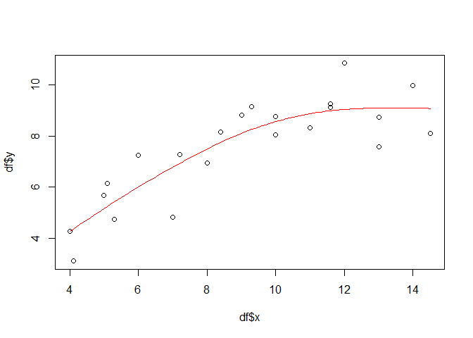
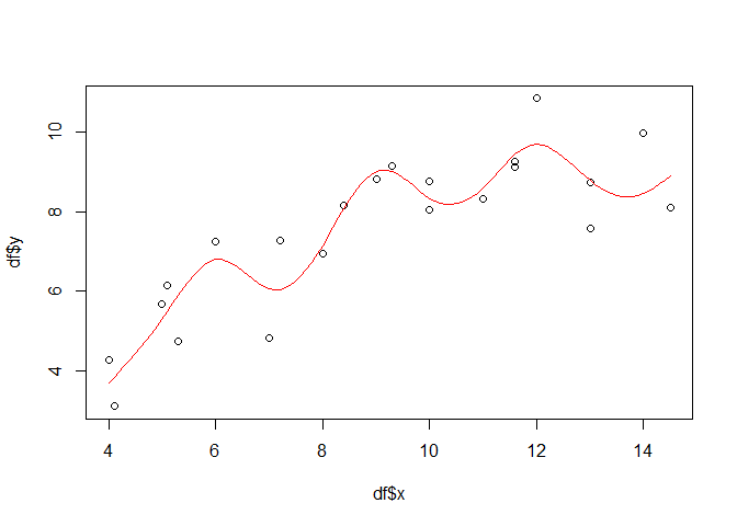
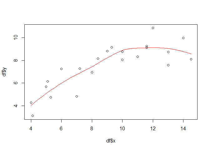
Obviously, there must be more than just swithing a function call to come from linear models to additive models. And there is: while for simple linear models, the equation would be something like y = a+bx, a smoothing term replace the slope b in additive models: y = a+s(x). By adding this term to the gam function and using a penalized regression spline (fx = FALSE which is the default), we finally get a first non-linear model:
gammod <- gam(y ~ s(x, fx = FALSE), data = df)

px <- seq(min(df$x), max(df$x), 0.1)
gampred <- predict(gammod, list(x = px))

plot(df$x, df$y)
lines(px, gampred, col = "red")
summary(gammod)
##
## Family: gaussian
## Link function: identity
##
## Formula:
## y ~ s(x, fx = FALSE)
##
## Parametric coefficients:
##             Estimate Std. Error t value Pr(>|t|)
## (Intercept)   7.5009     0.2108   35.58   <2e-16 ***
## ---
## Signif. codes:  0 '***' 0.001 '**' 0.01 '*' 0.05 '.' 0.1 ' ' 1
##
## Approximate significance of smooth terms:
##        edf Ref.df     F  p-value
## s(x) 2.243  2.792 22.94 3.06e-07 ***
## ---
## Signif. codes:  0 '***' 0.001 '**' 0.01 '*' 0.05 '.' 0.1 ' ' 1
##
## R-sq.(adj) =  0.751   Deviance explained = 77.8%
## GCV = 1.1471  Scale est. = 0.97807   n = 22
A look on the model performance reveils that the explained deviance has increased. Assuming that all model assumptions, which are actually the same as for linear models (except the linear relationship) are met, the explained deviance has increased to almost 78 percent. In order to check the model assumptions, you can use e.g. the gam.checked function.
gam.check(gammod)
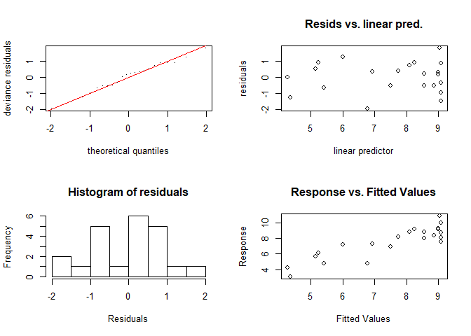
##
## Method: GCV   Optimizer: magic
## Smoothing parameter selection converged after 5 iterations.
## The RMS GCV score gradient at convergence was 9.91457e-07 .
## The Hessian was positive definite.
## Model rank =  10 / 10
##
## Basis dimension (k) checking results. Low p-value (k-index<1) may
## indicate that k is too low, especially if edf is close to k'.
##
##        k'  edf k-index p-value
## s(x) 9.00 2.24    1.48    0.97
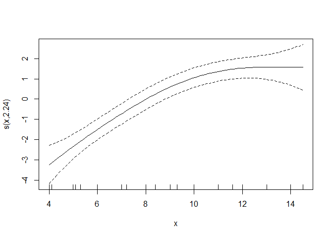
Speaking of side notes: this is how you can visualize the smoother quickly (you have to add the intercept to get the final prediction values):
plot(gammod)
Optimal smoother selection and reducing the risk of overfitting
One might wonder, why this and no other smoother has been found in the end. The reason relies in the way, the default penalized regression works (which is beyond the scope of this example but to sum it up: the regression penalizes each added smoothing term, i.e. each reduction in the resulting degrees of freedom of the model). To illustrate what would happen if no penalized but just a simple spline regression would be used, one can set the fx option to TRUE:
gammod <- gam(y ~ s(x, bs = "tp", fx = TRUE), data = df)

px <- seq(min(df$x), max(df$x), 0.1)
gampred <- predict(gammod, list(x = px))

plot(df$x, df$y)
lines(px, gampred, col = "red")
summary(gammod)
##
## Family: gaussian
## Link function: identity
##
## Formula:
## y ~ s(x, bs = "tp", fx = TRUE)
##
## Parametric coefficients:
##             Estimate Std. Error t value Pr(>|t|)
## (Intercept)   7.5009     0.2155    34.8 2.02e-13 ***
## ---
## Signif. codes:  0 '***' 0.001 '**' 0.01 '*' 0.05 '.' 0.1 ' ' 1
##
## Approximate significance of smooth terms:
##      edf Ref.df     F  p-value
## s(x)   9      9 7.643 0.000904 ***
## ---
## Signif. codes:  0 '***' 0.001 '**' 0.01 '*' 0.05 '.' 0.1 ' ' 1
##
## R-sq.(adj) =   0.74   Deviance explained = 85.1%
## GCV = 1.8733  Scale est. = 1.0218    n = 22
Now the function is highly non-linear and 9 degrees of freedom are used for the smooth terms. The explained deviance has increased but overfitting is very likely (the R squared has declined, too, but we should not give to much emphasis on that).
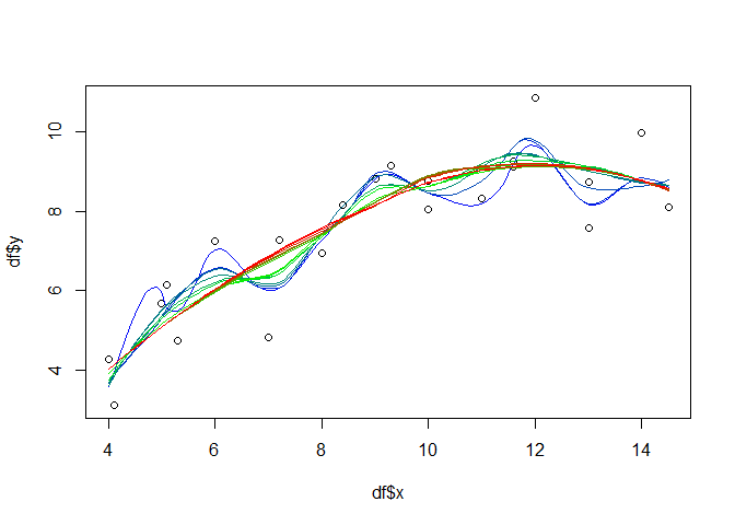
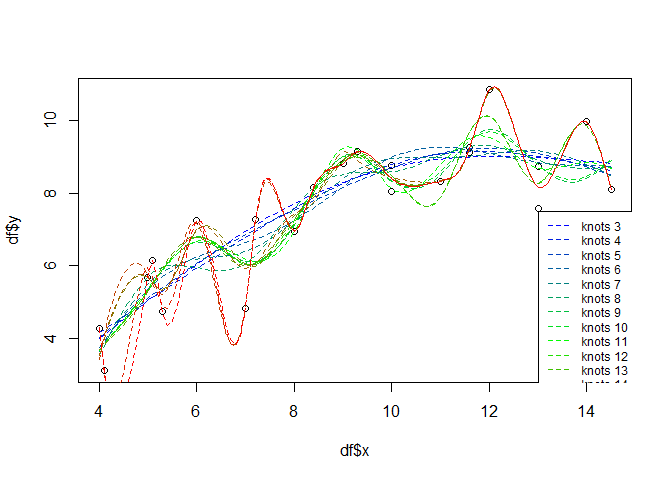
If you do not want to use the standard (penalty) model selection, a feasible approach for the additive models might be to select the number of knots and iterate over them in e.g. a leave-many-out cross validation approach. For illustration purposes, the following will just show the iteration and visualize the different model results in one plot:
knots <- seq(3, 19)

palette <- colorRampPalette(colors=c("blue", "green", "red"))
cols <- palette(length(knots))

plot(df$x, df$y)

for(i in seq(length(knots))){
  gammod <- gam(y ~ s(x, k = knots[i], fx = TRUE), data = df)
  px <- seq(min(df$x), max(df$x), 0.1)
  gampred <- predict(gammod, list(x = px))
  lines(px, gampred, col = cols[i], lty=2)
}

legend(13, 7.5, paste("knots", knots, sep = " "), col = cols, lty=2, cex=0.75)
LOESS
While the above examples are more straight forward if one comes from the implementation side of a linear model (i.e. lm), the locally weighted scatterplot smoothing (LOESS) is more straight forward from a conceptual point of view. It uses local linear regressions defined on moving subsets of the data set. For example, if the moving window is set to 21 pixels, than only the 10 left and right neighbours of the actually considered value (target) are considered and a linear regression is computed based on this subset. The term weighted indicates that not all of the neighbouring pixels are equally treated but the ones closer to the target are weighted higher. The following shows one example using 75 percent of all the data pairs in order to compute the local regression for each target value:
loessmod <- loess(y ~ x, data = df, span = 0.75)

px <- seq(min(df$x), max(df$x), 0.1)
loesspred <- predict(loessmod, data.frame(x = px), type = "response")

plot(df$x, df$y)
lines(px, loesspred, col = "red")
Again, one could iterate over the window size in a e.g. cross-validation approach to identify the best fit. As for the gam model, the following just illustrates the different models:
window <- seq(0.3, 1, 0.01)

palette <- colorRampPalette(colors=c("blue", "green", "red"))
cols <- palette(length(window))

plot(df$x, df$y)

for(i in seq(length(window))){
  loessmod <- loess(y ~ x, data = df, span = window[i])
  px <- seq(min(df$x), max(df$x), 0.1)
  loesspred <- predict(loessmod, data.frame(x = px))
  lines(px, loesspred, col = cols[i])
}