Cross-validation
Test statistics can describe the quality or accuracy of regression models if the assumptions of the models are met. However, the assessment would still be based on a model that is perfectly fitted to a given sample. To assess the prediction performance of a model in a more independent manner, the accuracy must be computed based on an independent (sub)-sample.
The straight-forward way for a test on an independent sample is of course the one which actually fits the model on sample A and tests it on a completely different sample B. However, in real-world applications, the required sample size is not sufficient in many cases. Therefore, cross-validation - althgough not entierly independent - is a good alternative to get an idea of the model performance for data values which have not been part of the fitted model.
In principal, there are two strategies for cross-validation:
-
Leave-one-out cross-validation: in this case, one value pair or data point of the sample data set is left out during model fitting and the model accuracy is estimated based on the quality of the prediction for the left-out value. In order to obtain a sufficiently large sample size, this procedure is iterated over all value pairs of the data set (i.e. each data point is left out once).
-
Leave-many-out cross-validation: in this case, more than one value pair or data point of the sample data set is left out during model fitting and the model accuracy is estimated based on the quality of the prediction for the left-out samples. This strategy is suitable for larger data sets, in which e.g. 80% of the data can be used as training data for fitting and 20% can be used as independent data for validation. The procedure can of course be repeated by creating models for different random training data sets and testing them using the respective left-out samples. Please note that independency is compromised to a small degree in the latter case. On the other hand, one can get a better impression of the model performance, especially if the different validation data sets are not averaged but used independently for geting an idea of the variation of the performance.
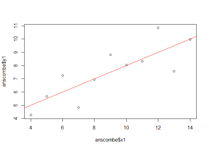
To illustrate the concept of cross-validation, we stay with the anscombe dataset
and use x1 and y1 as independent and dependent variable, respectively.
The statistics of a linear regression model would be:
lmod <- lm(y1 ~ x1, data = anscombe)

plot(anscombe$x1, anscombe$y1)
abline(lmod, col = "red")
anova(lmod)
## Analysis of Variance Table
##
## Response: y1
##           Df Sum Sq Mean Sq F value  Pr(>F)
## x1         1 27.510 27.5100   17.99 0.00217 **
## Residuals  9 13.763  1.5292
## ---
## Signif. codes:  0 '***' 0.001 '**' 0.01 '*' 0.05 '.' 0.1 ' ' 1
summary(lmod)
##
## Call:
## lm(formula = y1 ~ x1, data = anscombe)
##
## Residuals:
##      Min       1Q   Median       3Q      Max
## -1.92127 -0.45577 -0.04136  0.70941  1.83882
##
## Coefficients:
##             Estimate Std. Error t value Pr(>|t|)
## (Intercept)   3.0001     1.1247   2.667  0.02573 *
## x1            0.5001     0.1179   4.241  0.00217 **
## ---
## Signif. codes:  0 '***' 0.001 '**' 0.01 '*' 0.05 '.' 0.1 ' ' 1
##
## Residual standard error: 1.237 on 9 degrees of freedom
## Multiple R-squared:  0.6665,	Adjusted R-squared:  0.6295
## F-statistic: 17.99 on 1 and 9 DF,  p-value: 0.00217
Leave-one-out cross-validation
For the leave-one-out cross-validation, the training sample is comprised by all but one value pairs of the data set and the left-out data pair is used as validation sample. The procedure is typically iterated over the entire data set, i.e. each value is left-out once.
# Leave one out cross-validation
cv <- lapply(seq(nrow(anscombe)), function(i){
  train <- anscombe[-i,]
  test <- anscombe[i,]
  lmod <- lm(y1 ~ x1, data = train)
  pred <- predict(lmod, newdata = test)
  obsv <- test$y1
  data.frame(pred = pred,
             obsv = obsv,
             model_r_squared = summary(lmod)$r.squared)
})
cv <- do.call("rbind", cv)

ss_obsrv <- sum((cv$obsv - mean(cv$obsv))**2)
ss_model <- sum((cv$pred - mean(cv$obsv))**2)
ss_resid <- sum((cv$obsv - cv$pred)**2)

mss_obsrv <- ss_obsrv / (length(cv$obsv) - 1)
mss_model <- ss_model / 1
mss_resid <- ss_resid / (length(cv$obsv) - 2)

plot(cv$obsv, (cv$obsv - cv$pred))
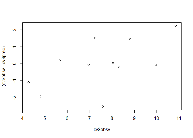
Based on this example, one could compute something like the F and r-squared values of an anova. Notably, compared to the “internal” F-test of the anova from the original model and the r-squared value, the cross-validation indicates a less accurate prediction.
data.frame(NAME = c("cross-validation F value",
                    "linear model F value",
                    "cross-validation r squared",
                    "linear model r squared"),
           VALUE = c(round(mss_model / mss_resid, 2),
                     round(anova(lmod)$'F value'[1], 2),
                     round(1 - ss_resid / ss_obsrv, 2),
                     round(summary(lmod)$r.squared, 2)))
##                         NAME VALUE
## 1   cross-validation F value 12.43
## 2       linear model F value 17.99
## 3 cross-validation r squared  0.50
## 4     linear model r squared  0.67
The range of r-squared values from the individual cross-validation models is computed by
max(cv$model_r_squared) - min(cv$model_r_squared)
summary(cv$model_r_squared)
and yields
## 0.219664
##    Min. 1st Qu.  Median    Mean 3rd Qu.    Max.
##  0.5640  0.6482  0.6640  0.6668  0.6915  0.7836
Aside from this error metric, a variety of different error metrics is commonly used to describe the predictive performance of a model (for regression-based approaches):
se <- function(x) sd(x, na.rm = TRUE)/sqrt(length(na.exclude(x)))

me <- round(mean(cv$pred - cv$obs, na.rm = TRUE), 2)
me_sd <- round(se(cv$pred - cv$obs), 2)
mae <- round(mean(abs(cv$pred - cv$obs), na.rm = TRUE), 2)
mae_sd <- round(se(abs(cv$pred - cv$obs)), 2)
rmse <- round(sqrt(mean((cv$pred - cv$obs)^2, na.rm = TRUE)), 2)
rmse_sd <- round(se((cv$pred - cv$obs)^2), 2)

data.frame(NAME = c("Mean error (ME)", "Std. error of ME",
                    "Mean absolute error (MAE)", "Std. error of MAE",
                    "Root mean square error (RMSE)", "Std. error of RMSE"),
           VALUE = c(me, me_sd,
                     mae, mae_sd,
                     rmse, rmse_sd))
##                            NAME VALUE
## 1               Mean error (ME)  0.04
## 2              Std. error of ME  0.43
## 3     Mean absolute error (MAE)  1.03
## 4             Std. error of MAE  0.29
## 5 Root mean square error (RMSE)  1.37
## 6            Std. error of RMSE  0.68
Leave-many-out cross-validation
For the leave-many-out cross-validation, the following example computes 100 different models. For each model, a training sample of 80% of the data set is randomly chosen.
range <- nrow(anscombe)
nbr <- nrow(anscombe) * 0.8

cv_sample <- lapply(seq(100), function(i){
  set.seed(i)
  smpl <- sample(range, nbr)
  train <- anscombe[smpl,]
  test <- anscombe[-smpl,]
  lmod <- lm(y1 ~ x1, data = train)
  pred <- predict(lmod, newdata = test)
  obsv <- test$y1
  resid <- obsv - pred
  ss_obsrv <- sum((obsv - mean(obsv))**2)
  ss_model <- sum((pred - mean(obsv))**2)
  ss_resid <- sum((obsv - pred)**2)
  mss_obsrv <- ss_obsrv / (length(obsv) - 1)
  mss_model <- ss_model / 1
  mss_resid <- ss_resid / (length(obsv) - 2)
  data.frame(pred = pred,
             obsv = obsv,
             resid = resid,
             ss_obsrv = ss_obsrv,
             ss_model = ss_model,
             ss_resid = ss_resid,
             mss_obsrv = mss_obsrv,
             mss_model = mss_model,
             mss_resid = mss_resid,
             r_squared = ss_model / ss_obsrv
  )
})
cv_sample <- do.call("rbind", cv_sample)

ss_obsrv <- sum((cv_sample$obsv - mean(cv_sample$obsv))**2)
ss_model <- sum((cv_sample$pred - mean(cv_sample$obsv))**2)
ss_resid <- sum((cv_sample$obsv - cv_sample$pred)**2)

mss_obsrv <- ss_obsrv / (length(cv_sample$obsv) - 1)
mss_model <- ss_model / 1
mss_resid <- ss_resid / (length(cv_sample$obsv) - 2)
Other error metrics for describing the performance of the prediction:
data.frame(NAME = c("cross-validation F value",
                    "linear model F value",
                    "cross-validation r squared",
                    "linear model r squared"),
           VALUE = c(round(mss_model / mss_resid, 2),
                     round(anova(lmod)$'F value'[1], 2),
                     round(1 - ss_resid / ss_obsrv, 2),
                     round(summary(lmod)$r.squared, 2)))
##                         NAME  VALUE
## 1   cross-validation F value 403.81
## 2       linear model F value  17.99
## 3 cross-validation r squared   0.48
## 4     linear model r squared   0.67
Aside from that, a variety of different errors is commonly used to describe the predictive performance of the model (for regression based approaches):
se <- function(x) sd(x, na.rm = TRUE)/sqrt(length(na.exclude(x)))

me <- round(mean(cv_sample$pred - cv_sample$obs, na.rm = TRUE), 2)
me_sd <- round(se(cv_sample$pred - cv_sample$obs), 2)
mae <- round(mean(abs(cv_sample$pred - cv_sample$obs), na.rm = TRUE), 2)
mae_sd <- round(se(abs(cv_sample$pred - cv_sample$obs)), 2)
rmse <- round(sqrt(mean((cv_sample$pred - cv_sample$obs)^2, na.rm = TRUE)), 2)
rmse_sd <- round(se((cv_sample$pred - cv_sample$obs)^2), 2)

data.frame(NAME = c("Mean error (ME)", "Std. error of ME",
                    "Mean absolute error (MAE)", "Std. error of MAE",
                    "Root mean square error (RMSE)", "Std. error of RMSE"),
           VALUE = c(me, me_sd,
                     mae, mae_sd,
                     rmse, rmse_sd))
##                            NAME VALUE
## 1               Mean error (ME)  0.06
## 2              Std. error of ME  0.08
## 3     Mean absolute error (MAE)  1.12
## 4             Std. error of MAE  0.05
## 5 Root mean square error (RMSE)  1.42
## 6            Std. error of RMSE  0.13